The Geostatistical Software Tool Program: Overview and some Highlighted Features.

Vladimir A. Maltsev.

VNIIGEOSYSTEM Institute, 113105, Varshavskoye shosse 8, Moscow, Russia.

E-mail:† vl-maltsev@yandex.ru.

Abstract. The Geostatistical Software Tool is the leading block modeling software in Russia. ItТs in use since 1990 and is installed in dozens of geological, mining, scientific, educational organizations. Main applications are: block modeling in ore estimation, expert analysis of the mining projects, studying the applied geostatistics. The concept is to have a software without automation, but with a lot of transparent Ai, providing total manual control on everything, but one-click visual control, with the graphics interface, based on GIS technologies instead of usual CAD-like interface. When for educational or for expert problems, the software is used as stand-alone, and for the practical modeling the main usage is as a replacement of the geostatistical modules in various full circle mining softwares. The Geostatistical Software Tool offers several unique mechanisms, the most interesting are the concept of secondary weighting functions and the concept of hierarchical block conditions.

Keywords: Geostatistics, Ore estimation, GIS, Mining geology.

PACS: 91.10.Da, 91.35.

OVERVIEW

The Geostatistical Software Tool is an original Russian block modeling software, known since 1989 [Maltsev, 1991] and having some features in its interface and in geostatistical math different from what is usual in western programs. Currently itТs available in 3 releases: stand-alone release, built into the GIS Integro software, and the library release. The library release allows easy building it into any or mining softwares, and all the functions can work in 2 modes: when they receive and return all the data in memory and donТt provide any interface, and when they receive / return in memory only the source data and main controll data, but the intermediate models are kept in internal files, and all the main dialogue and graphics windows remain available. Currently the software exists as a 32-bit Windows application with up to 2 computing threads, but the 64-bit Windows version, supporting more parallel computing, is now developed. The software uses the openGL graphics. Supported language is only Russian, but if enough interest appears, other languages also may appear.

GST uses its own database management. The source data, block models, solids and surfaces are importable/exportable. Block models may hold any quantity of properties. Solids also can possess information vectors, characterizing their volume. The models are backwards linked. This means, that each variogram model УknowsФ its experimental variogram and its source data file and column. Each property of the block model also УknowsФ, what the data was used, what variogram was used, etc. This allows semi-automatic recalculation of a lot of things, if some intermediate model is changed. Still, nothing is totally automated, all the manual controls on everything stay available, all the things stay transparent. The software has no own printing support. Instead, the button УAdd to reportФ is available everywhere. The reports are formatted as RTF files, that are then to be processed in a word processor.

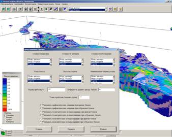
Figure 1.† The main window of the GST program.

The main window of GST is designed as a 3d GIS. Every visible object (sample, block, solid etc.) can be clicked to view or change its properties and to perform allowed operations. Controls on lighting, perspective, panning/mapping/rotating, sectioning, sizing of objects, color legends etc., are provided both from toolbars and keyboard shortcuts.

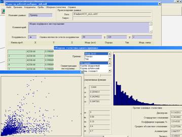
Figure 2.† The data editor of the GST program.

The source data editor has built-in tools for sorting, indexing, filtering, coordinate transforms, performing calculations, building logical masks, analyzing uni-variate and bi-variate statistics, up to non-linear correlations.

Non-usual operations, built into the source data editor are:

-       Locating and filtering out dublicate data;

-       Locating and filtering out closely located samples;

-       Clustering and declustering;

-       Building spatial measures of У density of samplingФ;

-       Finding blocks and solids to which samples belong;

-       etc.

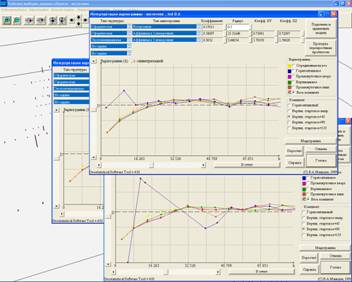
Figure 3.† The variography window of the GST program.

The variography engine is very different from what is found in other geostatistical softwares. Strictly speaking, itТs not just variography. Data transforms, trend analysis, part of declusterization, experimental variograms calculation, fitting of models, cross validation and more other things go together. Variogram model, trend model, data transform model, declusterisation model, parameters of the search ellipsoid, lriging type, kriging strategy Ц are considered not as separate things, but as parts of the complete variability model, that is managed from one point.

The variography window has a graphics interface, controlling everything related, and its main advantage is that it has in this center point just a button for the cross validation. So, the user has possibilities to check via cross validation everything that he is doing with all the main models, on every step, without any additional loss of time. Other unique feature of the program is the automatic variogram fitter, running in full specter of modes from full automatic to full manual. Moreover, it even УunderstandsФ if the user rescales graphs, disables experimental points, swithes to other structural functions (madograms etc) for the best readability of experimental variograms, and involves all of this userТs vision into the fitting process.

Probably, the most interesting point of the variography is the concept of sets of experimental variograms. When we define the main directions of the ore body, 15 directional variograms at a time are built in all 3 main and all intermediate directions. The complete УcloudФ† of directional variograms is never displayed. Instead Ц there are formed sets in main and intermediate geological plains, and these sets appear on tabs of the window. Each variogram in the set also can be isolated. This switching from set to set allows the user to have understandable and transparent control on 3d variography, staying in regular 2d geologic understanding like Уwhat happens in the section, taken along the bodyФ. With this, all the operations are performed on the complete 3d УcloudФ.

The block modeling itself and the solid modeling itself are much closer to what is usually met. The first significant difference is that kriging УmodulesФ are more universal than usually. For example, ordinary kriging, universal kriging, multi gaussian kriging and some others are integrated together. Features appear automatically in accordance to what models are defined as parts of the total variability model.

Another rare feature is AI support while kriging is performed. The backround algorithm is able of:

-       dynamically adjust the ellipsoid size according to several priorities given in parameters Ц minimum and maximum of samples, filling maximum possible octants, etc. altogether, saving the log of these actions;

-       dynamically control problems with kriging system Ц Уweights burstsФ, singularities etc., simplifying the model, or additionally declustering data, or additionally adjusting the ellipsoid until the problem disappears, also saving the log of these events and actions;

As a result Ц the user never receives block models with holes in it, even if any kriging estimation is impossible for some block, the block still will be estimated using inverse distances.

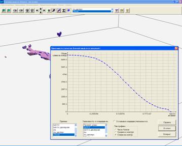
Figure 4.† The economical graphs in analysis of block models.

The kriging modules of the GST program are also able to operate with data, having faults or other structure breaking features. These features must be given as triangulated surfaces.

Available operations with block models are blocks filtering via mechanisms of primary conditions, secondary conditions and pseudo conditions (see in next sections), blocks filtering using solids and surfaces, arithmetical and logical operations on blocks and groups of blocks, mutual projections between block models and solids, manual manipulation with blocks, getting statistics on sets of blocks, calibrating of indicator probabilities, etc.

Some standard economical analysis end reserves computing tools are also enhanced. For example, concentration / reserve graphs may be drawn with or without conditioning of other important parameters.

So, the GST software is a very powerful and very cheap program tool in variography and block modeling, based on unique interface concepts [Maltsev, 1994]. The other modules (data base support, solids and surfaces construction, open pit optimizer) exist, but stay on some minimum necessary level. Enough for auditing, enough for educational, but not enough for practical mining. The main practical usage is using as a cheaper, more powerful, more controllable and more transparent replacement of geostatistical modules in large mining programs. In the former USSR itТs often used together with GEMS, Datamine, Surpack, Micromine and Samara softwares.

SECONDARY WEGHTING FUNCTIONS IN KRIGING

While geostatistical modeling, several problems can be met, where using some additional external data may appear useful. Of course, classical geostatistics provide possibilities of using external trends [Marechal, 1984], or external fuzzy parameters for markov-bayes kriging [Journel, 1986], but there are situations, where these tools arenТt enough. Mostly these situations refer to the case, when we need to use not an overall spatial property, but some relative measure for samples inside the search ellipsoid. In this case we can define a secondary weights property on our samples, with values in the (0,1) interval, that will be used in the following manner:

When we perform kriging for a block or a point with N samples in the area, we receive the kriging weights a1, a2,ЕaN, where a1+a2+Е+aN = 1. The secondary weights for the samples are w, w2,Е, w. We simply calculate new weighs as t*a1*w1, t*a2*w2Е t*aN*wN, where t is the Lagrange multiplier to provide t*a1*w1 + t*a2*w2 + Е† + t*aN*wN =1. Of course, we can insert these secondary weights and the second Lagrange multiplier directly into the kriging system, but this still remains for the future, actually because of that it becomes important only when we consider several secondary weighting properties, and yet we never used more than one.

The easiest way of understanding, how this mechanism works and what for it was designed, is to consider the three main application fields for it.

The Weighted Declustering of Data

When the sampling grid is highly irregular, clustering or declustering of the data is required. Mostly the necessity comes because of the geologists, that use to increase the density of sampling in rich localities and to decrease it outside these localities. As the result, systematic errors appear, raising our concentrations in a УlayerФ around dense localities, having thickness approximately the same as the search ellipsoid size. 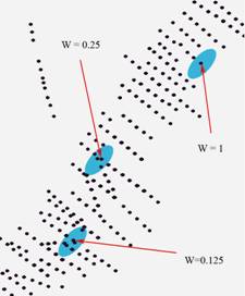If we use clustering of the data, we decrease the contrast of the spatial ore distribution, and if we use declustering, we lose a lot of our samples.

On the Fig.5 the scheme of the weighted declustering is presented. Secondary weights are calculates as a measure of the sampling density around each sample. The measure we use is 1/N, where N is the quantity of samples in the declustering ellipsoid, centered to the sample under consideration. The size of this declustering ellipsoid corresponds to the sampling network structure.

 

 

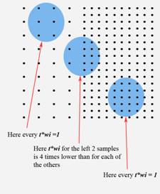
Figure 5. †How the secondary weights work as declustering weights. The scheme of generating the weights is at the left, the sheme of their usage in kriging is in the right. Both are 2d examples, while the real algorithm works in 3d.

 

Later, when the kriging is performed, these weights are applied as above. As one can see, in all the areas where the sampling density is uniform, both in dense areas and sparse areas, the resulting weights are exactly the same as the original kriging weights. The difference appears only where the search ellipsoid combines a part of a dense sampled area together with a part of a sparsely sampled area. In this case the weights of the УdenseФ samples are decreased, and the weights of the УsparseФ samples are increased. As the result Ц we use all the samples, we donТt lose the contrast, and we safely eliminate the bias, appearing from the sampling grid irregularities.

Of course, we must select the declustering ellipsoid geometry carefully, as everything in the applied geostatistics. Generally, its dimensions must be the same as the generalized sampling step in the sparsest area.

The УHurricane ConcentrationsФ

The problem of the Уhurricane concentrationsФ is a rather common thing for golden deposits, and even for some polymetallic deposits. If we do nothing to them, we receive biased estimations. The regular way is to replace concentrations upon some cutoff value by some lowered values. ItТs easy to understand the cutoff level itself, from which the concentrations may be considered as УhurricanesФ. For example, we can locate bending points on the cumulative histogram in the log scale of the data. ItТs less evident to understand, what to do then. To cut them to this limit? To cut them to averaged in the geological block? Anything else? ItТs also less evident to understand, whether they are real УhurricanesФ, or they are related to rich nests of considerable size.

There is no mistake in careful examination of each high value. If we know from some geological reasons, that we must expect rich nests, we must not consider any limitations of values. Instead, we must consider limitations on their Уinfluence zoneФ. Or Ц some limitations on kriging weights for the УhurricaneФ samples. Understanding the mechanism of the secondary weighted kriging, we can see, that limiting the influence zone and limiting of weights are very similar things, but the first one canТt be integrated into the kriging task, and the second one Ц can.

For example, on the Ridder polymetallic deposit (Kazakhstan) we know, that we expect nests of about 3x3x0.5 m, and the sampling network is 10x10x1 m. Each УhurricaneФ means such a nest. Previously these nests were estimated with separate solids. This was a terrific job, because Rigger is a huge deposit, containing thousands of such nests. 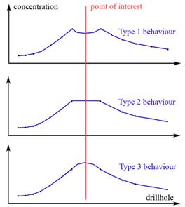Now we can build the secondary weighting function (like declustering weights), that equal to 1 in non-hurricane samples, and 0.3 in hurricane samples, and use it in kriging.

If we deal with a partially excavated deposit, like Ridder, we know exactly, what size of nests do we expect and we can properly calibrate the weighting function. If not, we still can use this approach with partial calibration:

-         If we deal with explorating with a mine and we can see geological regularities, we can use these regularities to calibrate the method.

-         If we deal with the drillhole data, we can examine pairs of neighboring intervals and understand something usable for calibration.

-         If not, we can try to validate it statistically, searching for the weighting divisor, that will show the maximum linearity of the estimated values / original values graph on the cross-validation.

-         If still no considerations appear, the 0.3 Ц 0.4 divisor is generally good for polymetallic deposits, 0.2 Ц 0.25 for golden deposits.

The method was used on about 25 various deposits, each time compared to the УregularФ schemes of limiting the УhurricanesФ. In all the cases the weighted approach appeared to be robust enough, so even the last way, without any calibration, seems to be good enough, not worse than the approach with limiting the values.

Weighting the Reliability for Samples

The original idea, that caused the secondary weighting tool to be designed, was to take the proper correction in case of an exploration system with different types of sampling.† The Zun-Kholba golden deposit was studied on several stages of exploration using drillholes of 3 diameters and using mine galleries. When excavation started, the reserves appeared to be strongly overestimated, there was an extended search for the reason, and the development of this tool was one of the search directions. The source of the mistake was found to be Уin the other fieldФ, but the tool appeared to be interesting and useful, secondary weighting the samples in the proportion of their physical weights, significantly increased the accuracy of kriging algorithms.

THE IMPROVED CROSS VALIDATION TECHNICS

Making difference to other geostatistical softwares, the cross validation tools in the GST program are built into the variogram fitting interface. Main ideas for this are:

-         The cross validation tests are to be performed each time we try even minor changes to our models.

-         The semi-automatic analysis of the cross validation results allows spending only several seconds on each test.

-         The cross-validation test integrates together all the models (trends, variograms, anisotropies, search ellipsoid size and behavior, kriging type and strategy, etc.) and leaves all of this as defaults for the kriging modules.

The Automated Cross Validation Tests

In most of the softwares the main cross validation result is just a table of estimated values for the locations of the source samples, and itТs recommended to start checking manually or semi-manually [Deutsch, Journel, 1992]:

-         Is there any spatial trend of errors?

-         Will the variogram of errors appear as a Уclear nugget effectФ variogram?

-         Is the value/error graph linear enough?

-         Is the estimation really unbiased?

All of these recommended tests can be automated completely, and itТs rather curious, why there is no one software, that does these tests in full automatic mode. Anyway, the GST does, and the results appear as warnings in the window of the AI support of kriging procedures.

The functionality of the AI support in cross validation and kriging algorithms also goes further and provides:

-         The Уweights burstФ monitoring. The effect appears because kriging doesnТt guarantee, that weights of 6 samples wouldnТt appear as something like +50, -50, 0.2, 0.2, 0,3, 0,3, and this may cause great problems. Possible origins of the effect are: (1) too complicated model (2) pairs of too closely located (3) improper search strategy. Possible actions are: (1) declustering of the data (2) simplifying of the model, (3) checking the search strategy (4) local automatic simplifying of the model. The cross validation and kriging modules in the GST program use AI to diagnose the weights burst for a block, and to simplify the variogram for this block or even to replace kriging for this block by anisotropic inverse distances if allowed by user.

-         The kriging system singularity actions. The GST is able to replace kriging estimation by anisotropic inverse distances estimation for the blocks, in which the kriging system is singular.

-         The automated minimum of samples correction. If performing kriging with trend (aka universal kriging), sometimes itТs a problem, that the search ellipsoid for some of the blocks doesnТt provide the quantity or the configuration of samples, needed for the requested trend model. The GST software is able to enlarge the search ellipsoid for these blocks, providing possibility of estimation.

-         The automated Уneed for krigingФ test. Actually, kriging must be used only when it provides better estimation than inverse distances, polyhedrons, or other simple estimation algorithms. The GTS cross validation modules test nit only kriging estimation, but also Уnearest sampleФ (almost the same as polyhedron) estimation and the inverse distances estimation, both using the same anisotropy as requested for kriging. Then the estimation statistics is analyzed, and the AI system gives the diagnosis, whether the kriging with current models actually works better, than simpler estimators.

The Scheme of Manual Cross Validation Tests

The main things for understanding the cross validation statistics are:

-         Even if the systematic error is statistically insignificant and the AI stays silent, its value shows us whether the source data needs clustering or declustering. The good check is to look on the bias of the cross-validation statistics before applying any data transform. Also the good idea is to check, what happens if to increase a bit the declustering grade.

-         The level of errors is the main question on how works the kriging we have got. But really this is the question Ц Уhow does it work on a bit sparser sampling gridФ? No really good criteria for the error levels is possible here. So, we leave the error levels analysis to the AI, relative to other estimators, and manually check, what happens to it when we change the models.

-         The same is for the correlation ratio. No good criteria on how high it must be, is possible. We just can Уpull a bitФ our model by each of the УhandlesФ, and see, whether it will grow or fall.

The improved scheme contains two more important tests. In next versions of the GST program - both would be moved to the automated testing system.

-         The nugget effect replacement. By definition, Уnugget effectФ relates to the ore regularities at radiuses, less than the sample size, or that are derived from the analysis artifacts. Actually, there may be regularities of larger size, not readable from the variogram, but rather important in kriging. Often itТs very useful to check, what happens if we replace the nugget effect with spherical or exponential model with very short radius, for example, half a metre. The quality of kriging in this case may increase dramatically. For example, the cross validation correlation ratio on the Zun-Holba golden deposit raised with this substitution from 0.19 to 0.49. Paradoxically, this approach works best when applied to golden deposits, where real nugget effect is classics. The cross validation test shows clearly, whether the substitution is needed. The complete study of what happens to the kriging estimators with such substitution and of how the kriging weights behave, can be found in [Babina, Maltsev, 2005].

-         The second significant thing, that is usually not readable from the variogram, not always evident from the geological view, and so the final decision may be taken via the automatable cross validation test, is the model function for the main structure. And the kriging is usually very sensitive to the selection of the type of the main structure, so this problem is of top importance. Some geological considerations of course also may be useful if we ask ourselves, how the ore must behave in the following case, but we canТt be always sure:

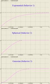
Figure 6.† The behavior of the 1-d kriging estimator on a Уflat peak in dataФ. On the left Ц main behaviour types (points are samples, line is estimator), on the right Ц corresponding variogram models

 

These 3 behaviours are defined by the main structure of the variogram behaviour near zero:

-         Behaviour 1 appears when the beginning part of the variogram is steeper than linear (i.e. exponential function);

-         Behaviour 2 appears when the the beginning part of the variogram is about linear (i.e. spherical function);

-         Behaviour 3 appears when the the beginning part of the variogram is lower than linear (i.e. Gaussian function);

If possible Ц these must be geological reasons for selecting. If there are no geological considerations, but there is enough data Ц cross-validation tests would clearly show the difference, significantly raising the correlation ratio. If still not sure Ц the first behavior is usually the selection for gold and alike, second for polymetallic ores, the third Ц for high-regular ores like gydrogenic uranium ores. Anyway, the test must be performed in any case.

DATA TRANSFORMS

The GST software has 3 mechanisms of using non-symmetrically distributed data. The first is the rather standard multi-gaussian approach [Verly, 1983], the second is the adoptive compensation approach, almost not known in the West, the third is the Уweights onlyФ approach, also rarely used in the West. The proper approach is usually selected only using the cross validation tests.

The Adoptive Compensation Approach

The method is described in [Maltsev, 1999], but briefly it is based on the following. Regular compensation for the back transform in log normal models is

†††††††††††††††††††††††††††††††††††††††††††††††††††††††††††††† †††††††††††††††††††††††††††††††††††††† (1)

where X is the estimation result in the log scale, Y is the result in the original scale; the variance is the variance of the log scale original data. This works when the distribution is really log normal. If it differs from the log normal even slightly, this correction stops working and may cause errors. This is why the usual log normal kriging is no more used.

If we consider another back transform correction, that in the log normal case is exactly the same as (1), but in another notation:

†††††††††††††††††††††††††††††††††††††††††††††††††††††††††††††† †††††††††††††††††††††††††††††††††††††† (2)

where M₁ is the mean of the source data, and M₂ is the mean of the log scale data, we receive estimation, which is much more robust to non-exactnesses of the log normal distribution.

Actually kriging is robust enough when working with symmetrical, but not normal distributions. This feature allows using the approach with any of KepteinТs distributions (becoming normal when transformed using some monotone non-linear function g). In this case the back transform becomes

†††††††††††††††††††††††††††††††††††††††††††††††††††††† †††††††††††††††††††††††††††††† (3)

where M₁ is the mean of the source data, and M₂ is the mean of the transformed data, g^-1 is the backward function to g.

The last is mostly needed because of often the distribution is far from both normal and log normal. In the West the regular practice is to use piecewise multi Gaussian transform, but some considerations show, that using polynomial KepteinТs distributions (root functions) may make more physical sense.

The mechanism of the normal distribution generation is an additive composition of enough uniform distributions. The mechanism of the log normal distribution generation is a multiplicative composition of enough uniform distributions.

And if not enough? If there are 3-5 of elementary distributions? In this case we receive a distribution that becomes symmetric and close to normal, if transformed through the root of corresponding power.

If we consider an ore deposit, in most of the cases weТll find its generation to be a result of breaking some thermodynamic equilibrium, and this equilibrium УhangsФ on a rather small quantity of the factors (3-10). Actually, this number is the number of factors that would interact in the multiplicative manner. This concept can possibly lead to understanding the proper data transform from the thermodynamic modeling, but yet it needs more studies.

The УWeights OnlyФ Approach

The method is described in [Maltsev, 1999]. Mathematically itТs absolutely incorrect, but surprisingly it works, and it was used in practical modeling of about 20 deposits.

The idea is trivial. All the variability model (variograms, trends, etc) are calculated and fitted using the transformed data. The weights of samples while kriging are also calculated for the transformed data. But then these weights are applied to normal scale data and there is no need for any back transform.

This approach also allows working not only with the log normal distribution, but with any KepteinТs distribution.

CONDITIONS AND PSEUDO CONDITIONS

When modeling a deposit, we always operate with sets of blocks, defined with some conditions. The GST program suggests specific tools for this.

At every moment some part of blocks appear as an active set. All the calculations are performed for this set. This set is defined by several tools, combined into a hierarchy.

On the lowest level we meet a tool of arithmetic conditions. Each property of the block model may have an arithmetic condition of УbelowФ or УaboveФ type. Only the blocks that meet all the conditions, that are defined, join the active set.

An additional tool on this level is a tool of Уsecondary arithmetic conditionsФ. These are used on multi-component deposits when we work with an arithmetic combination of concentrations. This condition defines a cut-off, below which a component will be ignored with the block model arithmetical processor, but does not directly affect the active set.

On upper levels we meet the mechanism of pseudo conditions. These are additional invisible properties in the block model, organized as values of triple logics. Possible values are -1, 0, 1 with the following meanings. If 0, then the block is qualified as on lower levels. If 1, then the lower level qualification is ignored, and the block is taken as active. If -1, then the lower level qualification is ignored, and the block is taken as non-active.

There are 4 independent pseudo conditions in the hierarchy. The first one is a geometrical pseudo condition. It receives information from solid models, whether a block belongs to a solid of interest or no. Actually, several pseudo conditions masks may be applied on this level, but they arenТt independent.

The second pseudo condition is a pseudo condition, based on economical considerations. Actually itТs rarely used because of lack of good ideas for building it.

The third pseudo condition is reserved for future needs.

The forth, highest pseudo condition is for technological masking. This is a pseudo condition, opened for manual editing directly from the 3d workspace of the program.

Of course, any pseudo condition may be cleared manually at any moment.

This hierarchy makes things flexible enough to try lots of variants of ore estimation, spending only seconds on each. Some of the advantages of this organization would be illustrated in the next section, that describes mechanisms if interactions between block models and solids models.

INTERACTIONS BETWEEN BLOCK MODELS AND SOLID MODELS

The GST program doesnТt work with geometry of solid models. Instead, it works with УprojectionsФ of the solid model into the block model. A solid model may contain several solids of Уtechnological typeФ, several solids of Уgeological typeФ, and several surfaces at once. Each projection operation is performed, using a set of Уactive solidsФ of same type, or several surfaces. Solids are considered not only as geometric boundaries, but as a holder of numerical data, specifying the space inside solid, so they posess vectors of numerical and logical data. A Уtechnological solidФ has a pre-defined Boolean property (i.e. ore/waste), and a vector of parameters, i.e. mean concentrations inside the solid or total reserves inside solid. A Уgeological solidФ has a numerical pre-defined property, something like rock codes. An unclosed surface may have only a binary property, saying whether itТs an upper surface or a lower surface.

Each surface or solid is just a set of non-ordered 3d-faces. No preliminary check on its topology is performed. The restrictions (checked only when a projection operation is performed) in a set of solids are:

-         parity of boundaries;

-         УgeologicalФ solids with different rock codes may not intersect, but may be enclosed;

-         УgeologicalФ solids of the same rock code are allowed to intersect, and are allowed to be enclosed, but not immediately (through a solid with some other rock code);

-         УtechnologicalФ solids of the same sign are allowed to intersect and are allowed to be enclosed;

-         УtechnologicalФ solids of different sign may not intersect but may be enclosed.

One thing here can cause ambiguous interpretation, so must be formulated clearly. If a sewing line intersects УtechnologicalФ solids, and sequential boundaries are of the same sign, then:

-         If they belong to one solid, they are interpreted as in-out.

-         If they belong to different solids, they are interpreted as enclosed one sign solids and the inner one is ignored.

No other checks are performed except listed above. The checks are performed only on sewing lines. If the ore body bifurcates, one can just leave two intersected, based on the same 3d ring. If the solids have gaps between faces, minor improperties, or even several missing faces, usually itТs possible to make them work by selecting a compliant sewing direction.

This approach allows using without problems imported solids that were prepared in almost any software via almost any methods, and even slightly incorrect solids.

Projections between Block Model and Solids Model

The first type of solids-to-blocks projection is preparing of a geometric pseudo condition. There are 3 modes for this operation. The first is to include into the active block set all the blocks that belong to active solids. The second is to remove from the active block set all the blocks that donТt belong to active solids. The third is to leave in the active block set all the blocks and only the blocks that belong to active solids. If the operation is performed with УtechnologicalФ solids, signs are resolved automatically. With УgeologicalФ solids Ц the active sets of solids may contain only solids of the same rock code. With surfaces Ц blocks not inside or outside, but upon or below active surface are qualified in the same manner. Several sequential operations on projections to the geometric pseudo condition are sequentially overlayed, the order is important.

The second type of solids-to-blocks projection is creating a new property in the block model, filled with any Boolean or numerical property from solids that stays undefined outside solids and is filled with a value from the information vector of the solid inside.

The third type of solids-to-blocks projection is creating a new property in the block model, filled with actual volumes of blocks that are inside a УtechnologicalФ solid, or with actual percentage of the block volume inside solid. Having several such properties for different kinds of solids allows solving rather complicated problems using the block model arithmetical/logical processor. For example, when re-estimating reserves on the Maleevskoye polymetallic deposit (Kazakhstan) 7 kinds of solids were used to define ore blocks, excavated volumes, etc., all huge (millions of triangles), all intersecting, with tasks like Уblocks must belong to solids sets A and B, not belong to C, or belong to D if belong to E, and all of this was resolved without any problems even with large blocks (10x10x2.5 m). This kind of projection uses sewing algorithm, up to 10x10 sewing lines in a block with smooth measuring along lines.

The backwards task (blocks-to-solids projection) is also supported. In this task each active solid receives a weighted mean or a sum of a specified property that will be calculated for blocks inside (or partially inside) the solid. The task also has several modes, the blocks that arenТt active, but belong to the solid, may join the calculation or may be ignored, an arithmetic property of the block model may be converted to Boolean and projected to the УgeologicalФ solid, etc.

So, both block models and solids models are used as spatial data transport and spatial data storage and are mutually convertible, and this makes a huge difference to most of the other geostatistical softwares, where solids are used only to restrict geometry and are mostly models of secondary importance. A lot of geologists prefer to operate numerical spatial data on the level of ore bodies, geological or excavation block, and not elementary blocks. Also, sometimes itТs rather useful to calculate, for example, the density of ore on a separate block model with larger blocks, integrate it to the solid model, averaging for ore bodies, an then spreading it to smaller blocks in the main block model. The thing, that isnТt evident to be good, but still is also rather useful, is that some kinds of solids may overlap, and some locations may belong to several solids, and are used for calculating integral characteristics of all the solids, containing them. This adds a lot of flexibility to the spatial modeling, but limits receiving general characteristics from the solid model. One can get these correct for each separate solid, but not for all the deposit, if not sure, that solids do not overlap.

Acknowledgments

The author wants to acknowledge all those who helped him in developing the software, who tested it, who allowed using their data for methodological studies, and who criticized the main concepts of it, personal thanks to Mikhail Katansky, Vladimir Kotkin, Alexander Tevelev and Tatyana Babina. †

References

1.† T.O.Babina, V.A.Maltsev, УMethods of improving effectivity of the kriging estimationsФ in Selected papers. 6-th Int. Conf. УNew ideas in Earth SciencesФ. Moscow, 2005.

2.† C.Y.Deutsch, A.G.Journel, УGSLIB: Geostatistical software library and userТs guideФ. NY, Oxford University Press, 1992.

3.† A.G.Journel, УConstrained interpolation and qualitative informationФ. in Math. Geology, 18(3). 1986, pp. 269-286.

4.† V.A.Maltsev, УPractical guide on using geostatistical estimation methods in geology, based on the GST softwareФ, Moscow, Geoinformmark, 1991, 109p.

5.† V.A.Maltsev, УMethods of software design for the controlled interpolation in geological tasksФ in Ores and Metals, Issue 1, Moscow, 1994, pp. 79 -89.

6.† V.A.Maltsev, УOn receiving unbiased estimations when modeling the ore deposits via nonlinear data transformsФ in Gornyi informacionno-geologicheskii bulletin, vol.5 (Ershov readings), Moscow, MGGA, 1999, pp. 106-111.

7.† V.A.Maltsev, УApplied geostatistics: technique of validating cutoff probabilities when solving the geometic task via indikator krigingФ in Understanding the genesis of ore deposits to meet the demands of the 21-th century. 12-th quadrennial IAGOD symposium. Moscow, 2006, pp. 89-90.

8.† G.Verly, УThe multi Gaussian approach and its applications to estimation of local reservesФ in Math. Geology, 15(2). 1983, pp. 259-286.

9.† A.Marechal, УKriging the seismic data in presence of faultsФ in G.Verly et. al., Geostatistics for natural resources characterization. Reidel, Dordcrecht, pp. 271-294.